In this article, we will show how to run IDclust on a Seurat object of a single- cell RNA dataset of the mouse brain from “Joint profiling of histone modifications and transcriptome in single cells from mouse brain,Chenxu Zhu, Yanxiao Zhang, Yang Eric Li, Jacinta Lucero, . Margarita Behrens, Bing Ren, Nature Methods, 2021 Paired-Tag”
Classical analysis of scRNA dataset with Seurat
Data
Download, extract & format scRNA of the mouse brain (Zhu et al., 2021) from the GEO portal.
set.seed(47)
# Download dataset
temp = tempfile()
tempdir = tempdir()
download.file("https://www.ncbi.nlm.nih.gov/geo/download/?acc=GSE152020&format=file&file=GSE152020%5FPaired%2DTag%5FRNA%5Ffiltered%5Fmatrix%2Etar%2Egz",
    temp, quiet = TRUE)
untar(temp, exdir = tempdir)

# Download metadata
annot = tempfile()
download.file("http://catlas.org/pairedTag/cellbrowser/Paired-tag/meta.tsv", annot,
    quiet = TRUE)
metadata = read.table(annot, sep = "\t", header = TRUE)
rownames(metadata) = metadata$Cell_ID

# Create Seurat object
datamatrix = Seurat::Read10X(file.path(tempdir, "01.Paired-Tag_seq_RNA_filtered_matrix"))
datamatrix = datamatrix[, match(metadata$Cell_ID, colnames(datamatrix))]
Seu = Seurat::CreateSeuratObject(datamatrix, assay = "RNA", meta.data = metadata)

# Subsample cells
Seu = Seu[, sample(ncol(Seu), 5000, replace = F)]
Seurat Analysis
We then run a classical Seurat normalization and dimensionality reduction. We can plot the UMAP and color by the cell type.
# From Seurat tutorial -
# https://satijalab.org/seurat/articles/pbmc3k_tutorial.html
Seu <- Seurat::NormalizeData(Seu, verbose = FALSE)
Seu <- Seurat::FindVariableFeatures(Seu, selection.method = "vst", nfeatures = 2000,
    verbose = FALSE)
Seu <- Seurat::ScaleData(Seu, verbose = FALSE)
Seu <- Seurat::RunPCA(Seu, features = Seurat::VariableFeatures(object = Seu), verbose = FALSE)
Seu <- Seurat::RunUMAP(Seu, reduction = "pca", dims = 1:50, verbose = FALSE)


Seurat::DimPlot(Seu, reduction = "umap", group.by = "Annotation")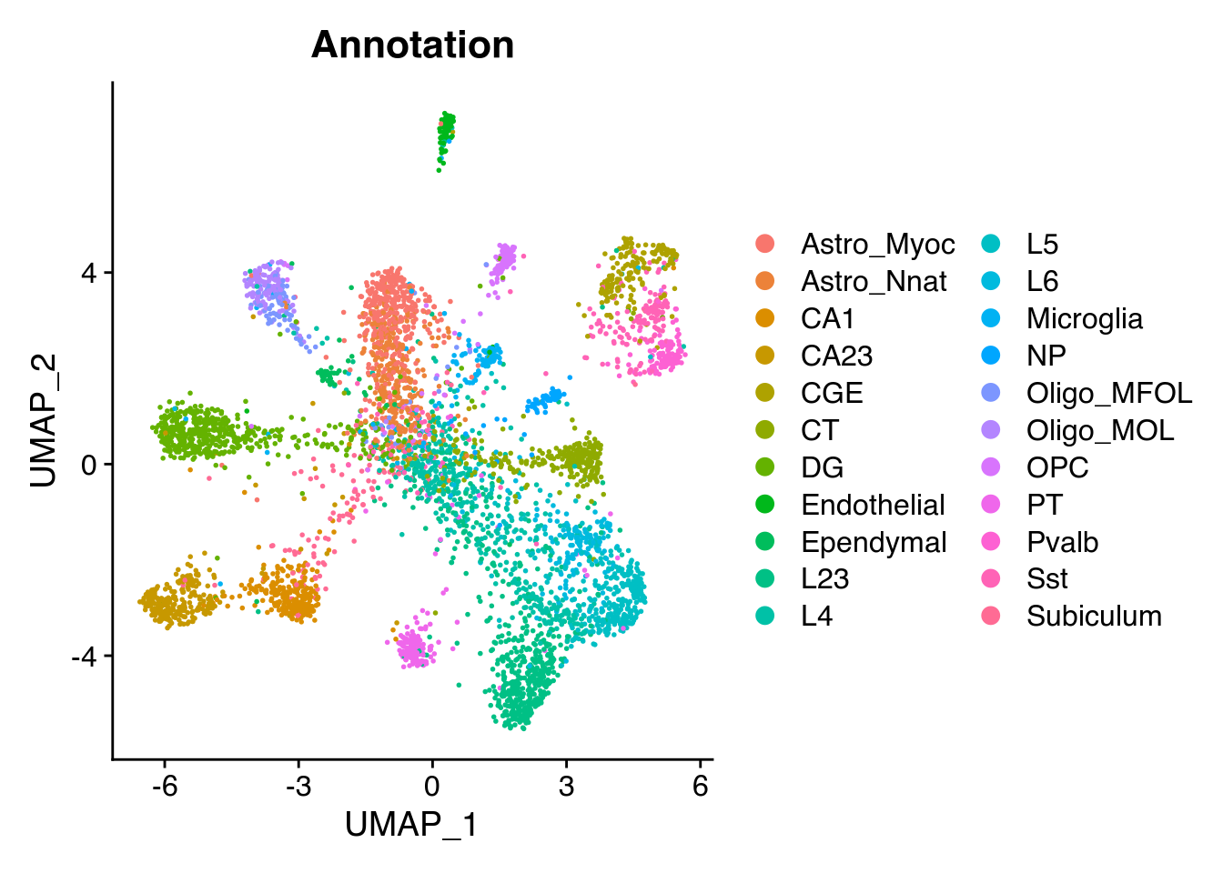
Classical Louvain clustering
We can run a classical Louvain clustering to see the clusters.
Seu <- Seurat::FindNeighbors(Seu, verbose = FALSE)
Seu <- Seurat::FindClusters(Seu, verbose = FALSE)

Seurat::DimPlot(Seu, reduction = "umap", group.by = "seurat_clusters")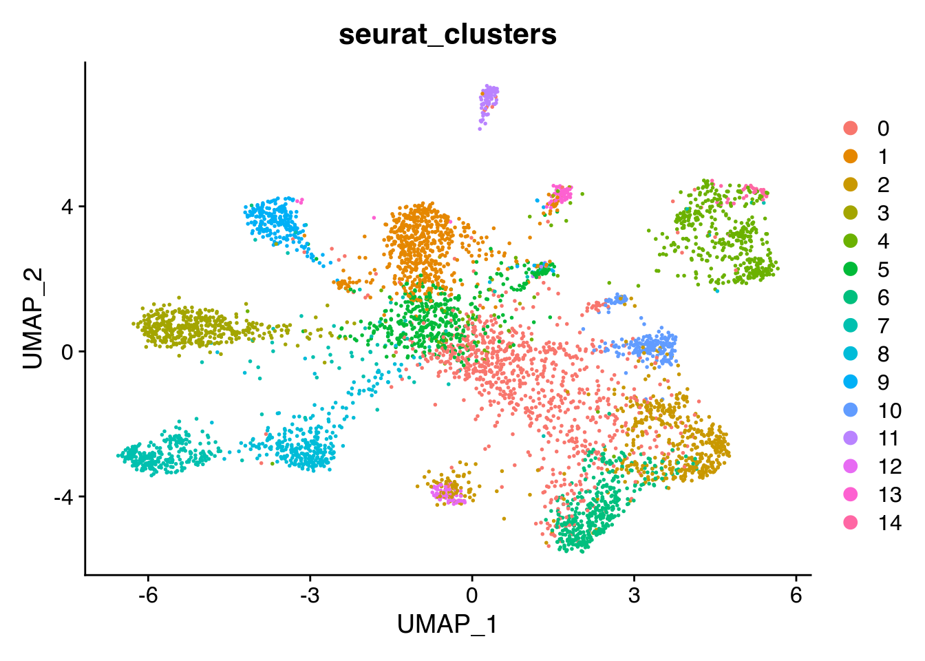
Iterative Differential Clustering
We can now run the Iterative Differential Clustering, that will re-process and re-cluster each cluster iteratively and find subclusters with significant differences between each other.
By default for a Seurat object the processing_Seurat function is used for re-processing and the differential_edgeR_pseudobulk_LRT is used to find significant marker genes.
set.seed(47)
output_dir = "~/Tests/IDC_Seurat/"
if (!dir.exists(output_dir)) dir.create(output_dir)
Seu = iterative_differential_clustering(Seu, output_dir = output_dir, plotting = FALSE,
    saving = TRUE, n_dims = 50, dim_red = "pca", vizualization_dim_red = "umap",
    processing_function = processing_Seurat, differential_function = differential_edgeR_pseudobulk_LRT,
    logFC.th = log2(1.5), qval.th = 0.01, min_frac_cell_assigned = 0.1, limit = 10,
    starting.resolution = 0.1, starting.k = 100, resolution = 0.8, k = 100, verbose = FALSE)
## Not enough cells to form 2 replicates ... assigning 0 differential genes.
## Not enough cells to form 2 replicates ... assigning 0 differential genes.We can now read in the output ‘IDC_summary’ object and plot the cluster hierarchies compared to the author clusters. On this plot, each node is a cluster. The colors represent the distribution of author cluster within each cluster. Link between nodes represent a hierarchy in the iteration. The width of the edges is proportional to the number of genes found.
IDC_summary = qs::qread(file.path(output_dir, "IDC_summary.qs"))
plot_cluster_network(Seu, IDC_summary = IDC_summary, node_size_factor = 4, color_by = "Annotation",
    legend = FALSE)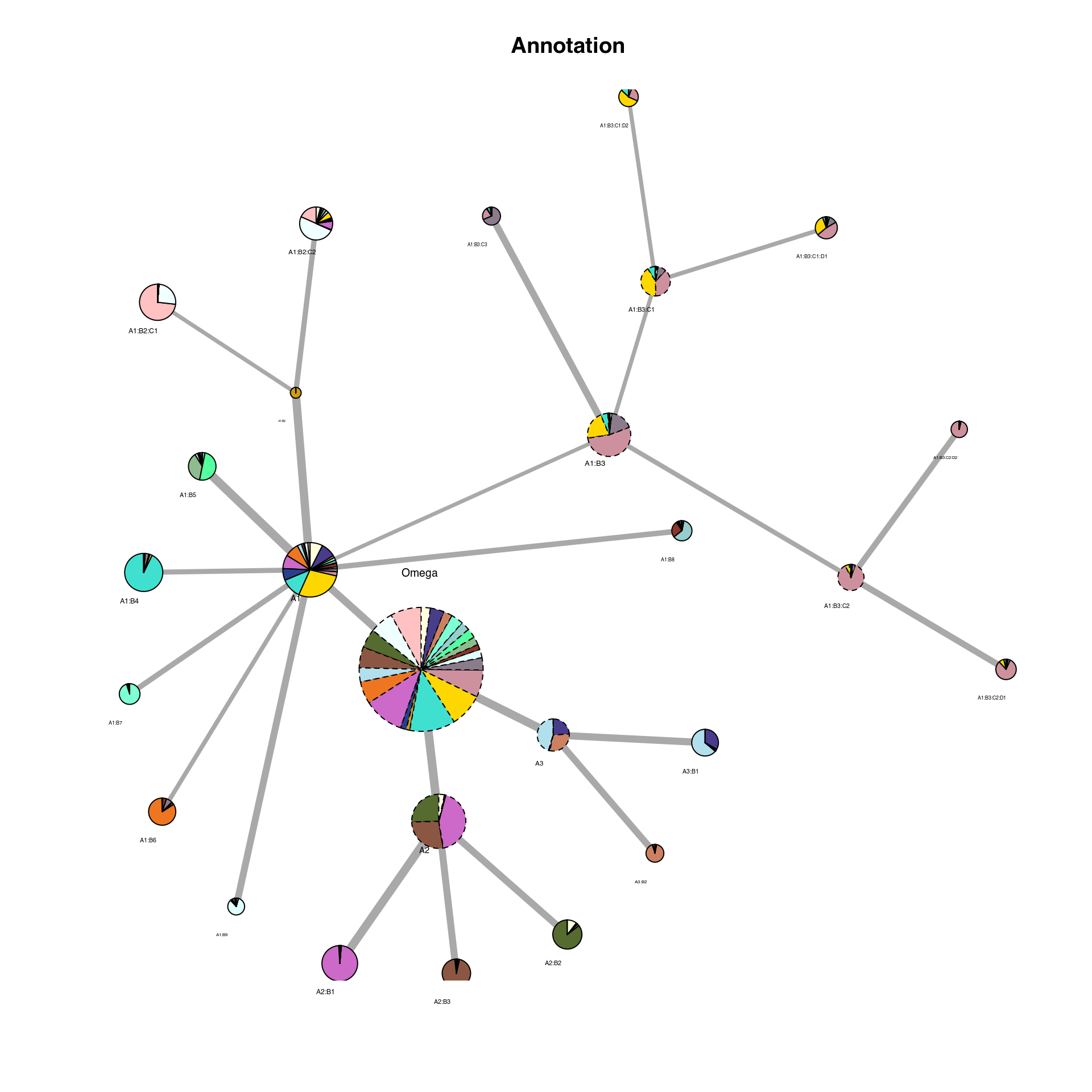
##     Annotation Annotation_color
## 1   Astro_Myoc       rosybrown1
## 2   Astro_Nnat            azure
## 3          CA1   darkolivegreen
## 4         CA23     lightsalmon4
## 5          CGE       lightblue2
## 6           CT       chocolate2
## 7           DG          orchid3
## 8  Endothelial       royalblue4
## 9    Ependymal       goldenrod3
## 10         L23        turquoise
## 11          L4             gold
## 12          L5            pink3
## 13          L6         thistle4
## 14   Microglia       lightcyan1
## 15          NP          tomato4
## 16  Oligo_MFOL     darkseagreen
## 17   Oligo_MOL        seagreen1
## 18         OPC   paleturquoise3
## 19          PT      aquamarine1
## 20       Pvalb     lightsalmon3
## 21         Sst    darkslateblue
## 22   Subiculum     lightyellow1
A ‘IDcluster’ column was added to the Seurat object, which we can now project the cluster found this way on the UMAP.
Seurat::DimPlot(Seu, reduction = "umap", group.by = "IDcluster")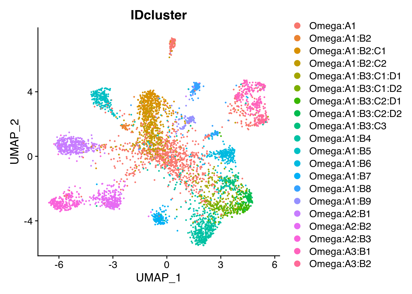
We can also plot particular marker genes in the cluster network by changing the ‘color_by’ parameter to a gene present in the Seurat object.
plot_cluster_network(Seu, IDC_summary = IDC_summary, color_by = "Erbb4", threshold_to_define_feature_active = 2,
    node_size_factor = 4, legend = FALSE)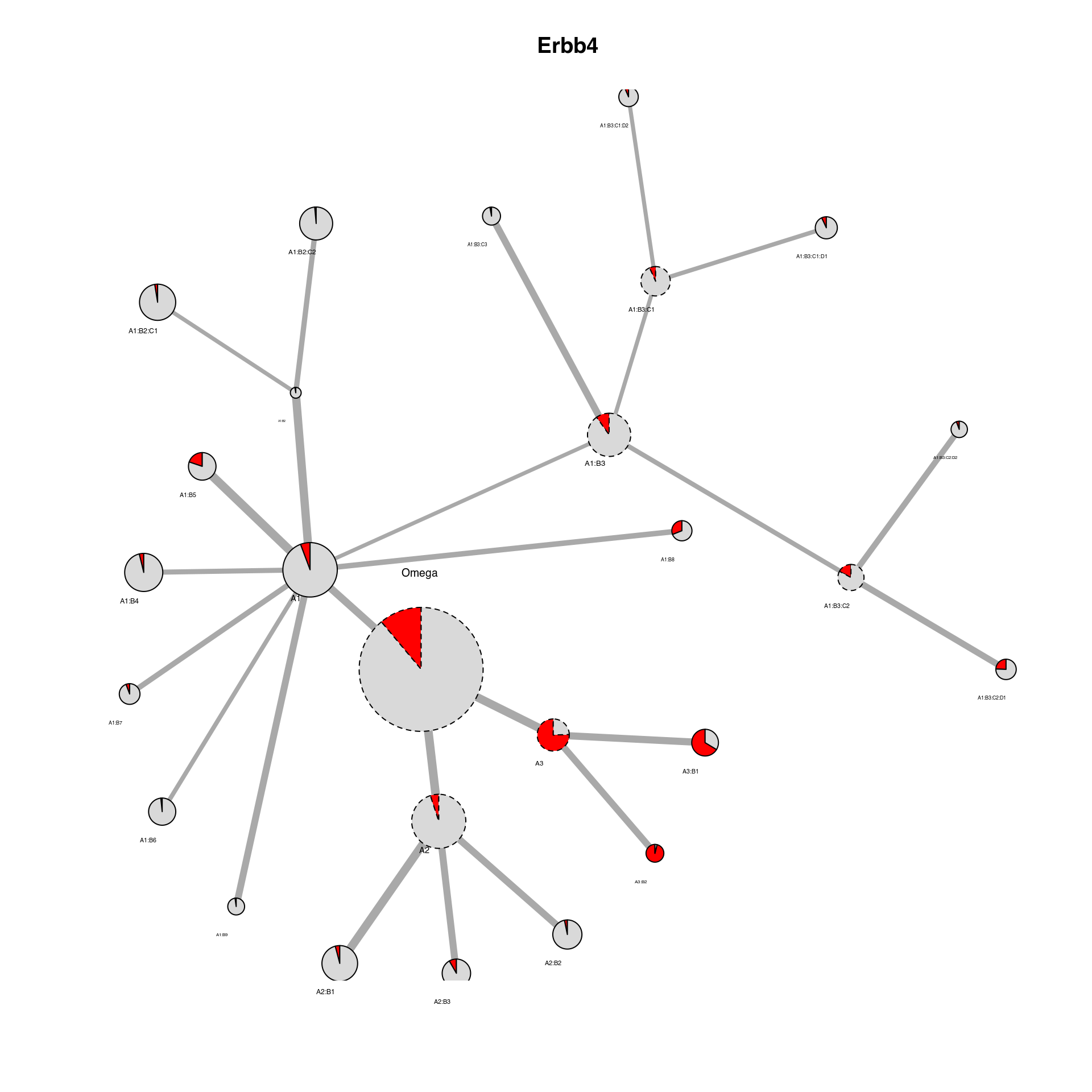
##      Erbb4 Erbb4_color
## 1   Active         red
## 2 Inactive      grey85